3 PASS Survey Design and Methodology - Weighting
Contact authors: Beste, Jonas; Trappmann, Mark.
Weighting constitutes an important part of the overall survey design and Methodology in PASS. Weighting methodology used in PASS ensures that survey estimates provide an unbiased representation of the target populations over time. Section 3.1 describes the construction of initial cross-sectional weights, including sample-design weights, non-response adjustments, and calibration procedures undertaken in the first wave. Section 3.2 explains how weights are updated for subsequent waves, detailing longitudinal weighting, the treatment of refreshment and replenishment samples, and adjustments for non-response and temporary drop-outs. Section 3.3 briefly discusses the integration of replenishment-sample weights into the ongoing panels. Section 3.4 summarises weighting datasets hweights (household weights) and pweights (person weights) and key variables they contain and their usage in analysis. Finally, Section 3.5 briefly describes the separate weighting scheme developed for the PASS web survey, which combines web-specific participation propensities with the existing PASS person weights to correct for selective web participation and to ensure comparability with the main survey.
3.1 Initial weighting process
PASS contains several sub-samples introduced across waves (see Section 2.1.5), including the initial welfare benefit (UB II)4 recipient and general population samples, annual refreshment samples for new UB II entrants, and replenishment samples in Waves 5, 11, and 17. Each sub-sample receives its own weights in the wave in which it first appears. Its construction consists of three stages:
3.1.1 Stage 1: Design weights for the gross sample
Design weights equal the reciprocal of the selection probability for the gross sample. Detailed description of the generation of these variables is provided in Rudolph & Trappmann (2007) and in wave-specific data reports for the replenishment samples (e.g., Berg et al. (2013), Berg et al. (2019), Anker et al. (2025), chapter 6.1 for wave 5,11 and 17 respectively).
Design weights are stored in the dataset hweights. The individual design weights supplied, and their meanings are provided in the table below:
This table lists design weight variables in the hweights dataset and explains their target populations.| Variable | Meaning |
|---|---|
| dw_ba | Design weight for welfare benefit recipient sample households (target population: households in which there was at least one benefit unit in joint receipt of benefits in accordance with Social Code Book II in any July since 2006) |
| dw_mi | Design weight for general population sample households (target population: households in the Federal Republic of Germany) |
| dw | Design weight for the combined sample (target population: households in the Federal Republic of Germany) |
3.1.2 Stage 2: Modelling non-response
Two logit models estimate the participation probability for all households in the gross sample:
Model 1: Predicts the probability of contact
Model 2: Predicts the probability of participation, conditional on contact (at least one household interview + ≥1 complete personal interview)
These models are estimated separately for each sub-sample.
The set of variables used in the above-mentioned propensity models have evolved during the first waves of PASS. In Wave 1, the general population sample model included micro-geographical indicators provided by Microm alongside regional characteristics such as federal state and municipality size. Full model specifications can be found in the wave-specific method reports (Hartmann et al. (2008); Büngeler et al. (2009); and data reports from 2011 to 2025, eg. Anker et al. (2025)).
For the UB II recipient samples5, additional characteristics on the level of the benefit unit from the sampling frames (A2LL and later XSozial) were included.
From Wave 3 onwards, Microm variables were dropped only variables on the level of benefit-unit, regional indicators, and the number of contact attempts were used for these samples. For the population replenishment samples age, gender and nationality were used in addition to regional predictors.
The product of the above-mentioned predicted probabilities from the two models is stored as prop_t0 variable in hweights dataset.
Design weights divided by estimated participation probabilities yield modified design weights, which are used in the calibration stage (see below).
3.1.3 Stage 3: Calibration
A detailed documentation of the calibration process for Waves 1 and 2 can be found in Kiesl (2010). The calibration procedures and results reported by TNS Infratest in the method and field reports (Hartmann et al., 2008); (Büngeler et al., 2009) do not correspond to the weights provided in the Scientific Use File. From Wave 3 onward, calibration procedures are described in the wave-specific data reports produced by infas (e.g. Anker et al. (2025)). We therefore outline only the core principles here. The focus below is on calibration for the initial Wave 1 samples, as refreshment samples in later waves were calibrated jointly with the full sample (see Sections 3.2.7 and 3.2.8).
Household-level calibration (Wave 1)
In the first step, both sub-samples and the combined total sample were calibrated to official household statistics.
Total and UB II sample weights for benefit recipients were aligned with benchmark statistics from the Federal Employment Agency (as per the monthly reporting of July 2006).
Total and Microm sample weights were additionally calibrated to private-household benchmark statistics for Germany (as per the annual reporting of 2007) from the Federal Statistical Office. These benchmark figures are documented in Kiesl (2010).
All PASS weights are household weights, whereas the BA benchmarks refer to benefit units. To align these levels, synthetic benefit units were created as described in the Wave 1 data report (see Christoph et al. (2008), p. 49; variable bgnr1 in p_register dataset). Households were first divided into synthetic benefit units, and calibration characteristics were generated at the benefit-unit level, including whether the unit received UB II at the sampling date. After calibration, multiplying these characteristics of benefit units in receipt of benefits, as of the sampling date, by household projection factors produced benchmark totals. All benefit units receiving benefits within the same household received identical projection factors.
Determining benefit-receipt of a household or even a benefit unit at the index date is not always straightforward. To support users, indicator variables are provided. For instance, the variable alg2samp at the household level is supplied in the hh_register dataset. This variable describes the benefit receipt as of the sampling date for all households in the categories:
0 - no receipt, 1 - receipt, 2 - no receipt according to survey (but included in UB II recipient sample and thus receipt according to register data), 3 - receipt unclear from survey (but included in UB II recipient sample and thus receipt according to register data), 4 - receipt unclear from survey (general population sample).
In addition, every user can generate this variable him/herself using the unemployment benefit II spell data (alg2_spells dataset). Other useful variables are AL20600 and AL20700a–o (describing the member/s in the household which receive benefits).
To generate the weights, it was imperative to determine which benefit units should be classified as receiving Unemployment Benefit II (UB II) at the sampling date. The following criteria were applied for this classification are as follows:
UB II recipient sample households (sample = 1)
All households drawn from the BA register were classified as receiving UB II at the sampling date, even if the respondent denied benefit receipt, provided at least one household member was aged between 15 and 64 years.
General population sample households (sample = 2)
In cases where survey data did not clearly establish benefit-receipt status, households were treated as receiving UB II for weighting purposes if both conditions held:
the household reported having ever received UB II (HA0300 = 1), and
the start or end date of at least one UB II spell fell in 2006 (including cases with unspecified start or end date).
Determining benefit receipt at the benefit-unit level presents greater uncertainty since it is not possible to obtain reliable retrospective data on benefit recipients in the household in July 2006. For most households, this is straightforward, as they consist of a single benefit unit that receives benefits if the household does. However, in households with multiple benefit units, determining benefit receipt becomes particularly difficult. So, the following procedure was applied:
Information pertaining to individuals within the household currently receiving benefits (AL20600 and AL20700a–o) was used.
A benefit unit was classified as receiving UB II if at least one of its members was reported as a benefit recipient.
In a household with more than one benefit unit and with no information as to which individuals the household is receiving benefits for (e. g. because the questionnaire responses state that no benefits are being claimed), all the synthetic benefit units were regarded as being in receipt of benefits.
This procedure results in the variable bgbezs1 in the p_register dataset.
The household-level calibrated weights derived from this process are stored in the hweights dataset:
wqbahh — calibrated household weight for the welfare benefit recipient sample
wqmihh — calibrated household weight for the general population sample
wqhh — calibrated household weight for the total sample
Individual-level calibration (Wave 1)
Following household-level calibration, individuals who completed a personal or senior citizen’s interview were calibrated to benchmark statistics at the person level. The calibrated household weights served as the starting point for this step.
The total and BA weights for benefit recipients in both sub-samples were calibrated to benchmark statistics from the Federal Employment Agency (as per the monthly reporting of July 2006). The total and general population sample weights were additionally calibrated to benchmark statistics from the Federal Statistical Office on private households in Germany for 2007. The benchmark figures used are detailed in Kiesl (2010).
Senior citizen’s interviews were calibrated to population statistics in the same way as standard personal interviews. However, the BA statistics do not contain figures on the number of senior citizens in households receiving benefits, nor do they identify individuals living in benefit-receiving households that are not part of a benefit unit. Consequently, it was not possible to obtain the BA person weights for these individuals by means of calibration.
Instead, we estimated the participation probability of these individuals, conditional on their household participating in the survey, using a logit model with the following covariates: number of individuals aged 15 and over in the household; interview mode; age; and gender. The modified design weight was subsequently divided by this value.
The calibrated person weights are contained in the pweights dataset:
wqbap — calibrated person weight of the UB II recipient sample
wqmip — calibrated person weight of the Microm sample
wqp — calibrated person weight of the total sample
3.2 Construction of the weights from wave 2 onwards
The starting point for the weighting procedure in wave 2, and for the longitudinal section from wave 1 to wave 2, is the set of cross-sectional household and individual weights from wave 1. More generally, for wave \(n+1\) and for the longitudinal section from wave \(n\) to wave \(n+1\) , the procedure begins with the cross-sectional weights from wave \(n\) for both households and individuals.
In wave \(n\) (\(n \ge 1\) ), each household has two weights: wqhh (the calibrated total weight) and depending on the sub-sample either wqbahh (calibrated UB II recipient sample weight) or wqmihh (calibrated general population weight). Similarly, each individual has two weights: wqp and depending on the subsample either wqbap (calibrated UB II recipient sample personal weight) or wqmip (calibrated general population personal weight). All four weights are updated for the subsequent wave (\(n+1\))
Figure 3.1 presents the steps in the weighting procedure, which are described in detail below. This section provides a general overview. From wave 3 onwards, chapter 6 in each wave-specific data report (e.g. Berg, Cramer, Dickmann, Gerber, et al. (2024)) documents the exact models, variables, and coefficients applied.
For wave 2, detailed documentation is available in Büngeler et al. (2009). This section does not discuss the integration of replenishment-sample weights into the ongoing panel; Section 3.3 addresses this topic in detail.
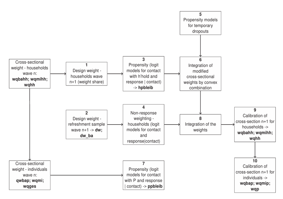
Figure 3.1: Generation of the weights for wave \(n+1\) given the weights of wave \(n\)
3.2.1 Design weights for the wave \(n\) households in the \(n+1\) th wave.
For wave \(n+1\) , new household design weights are generated from the wave \(n\) cross-sectional household weights, accounting for individuals moving into existing sample households from within Germany. This adjustment is carried out using a weight-share procedure.
Household events such as births, deaths, or moves out of the household do not affect the weight. By contrast, moves into a household from within Germany increases the inclusion probability, because these individuals also had a chance of being sampled in previous waves. Therefore, for the weighting calculations, when individuals move into a sample household from within Germany, the household’s prior inclusion probability is increased by the mean inclusion probability in the respective sub-sample (as the inclusion probabilities of the households in which new household members previously resided cannot be determined precisely for all earlier waves).
Consequently, the new design weight for sub-sample \(i\) \(dw_{i}hh_{n+1}\) is therefore calculated from the old cross-sectional weight \(wq_{i}hh_{n}\):
\[\frac{1}{dw_{i}hh_{n + 1}} = \frac{1}{wq_{i}hh_{n} + \,\left( \frac{n_{sample\, i}}{n_{population\, i}}\, \right)}\]
The new design weight is only an intermediate step and is therefore not included in the data.
3.2.2 Design weights for the wave \(n + 1\) refreshment sample
From wave 2 onwards, PASS draws an annual refreshment of the welfare benefit recipient (UB II) sample, selecting only benefit units (Bedarfsgemeinschaften) in which no member received benefits in July of the previous years. These refreshment samples are drawn from the same sampling points as the initial samples, with extensions to the 97 additional sampling points introduced in wave 5 and the 93 additional points added in wave 17.
Similar to the probability-proportional-to-size procedure used to draw the initial register data sample (Rudolph & Trappmann, 2007), the refreshment sample size in each sampling point is proportional to the share of new benefit recipients in the population at the time those sampling points were selected. The calculation of the design weights is further described in the same article. However, from wave 2 onwards, the number of benefit units within a household is no longer taken into account. The resulting design weight for refreshment sample is provided in the variable dw_ba for all cases.
3.2.3 Response propensity models for panel households
In this step, the probability of continued participation is estimated for each household that participated in the previous wave. This uses logit models capturing (1) panel consent, (2) risk of loss of contact, and (3) likelihood of refusal. These models include survey design features (e.g. interview mode, number of contact attempts), aspects of the previous interview (e.g. item non-response or partial non-response), household/respondent characteristics (e.g. gender, age, education, country of birth, labour force status, home ownership, household size), and area characteristics (e.g. municipality size), consistent with standard practice in longitudinal studies (Watson & Wooden, 2009).
The predicted propensities from the three models are multiplied. The reciprocal of this product is stored in the variable hpbleib, which serves two purposes:
The longitudinal weight of a household for the period \(wave_n\) ; \(wave_{n+k}\) between waves can then be calculated as the product of the cross-sectional weight for wave_n and the product of all hpbleib for wave \(n\) to wave \(n+k-1\).
The product of the updated household design weight from step 1 (see Section 3.2.2) multiplied by hpbleib (which we call “modified cross-sectional weight”) serves as a base for calculating a new cross-sectional weight for wave \(n+1\).
Note that this procedure works only for households with monotonous drop-out patterns and not for households that drop-out for one wave and return in the next wave. The treatment of those temporary drop-outs is specified in Section 3.2.5.
3.2.4 Non-response weighting for households in the wave n refreshment sample
For households drawn in the refreshment samples, non-response is modelled in a two-stage procedure, analogous to the approach used for the first wave. Full variable lists and model coefficients are documented in the respective wave-specific data reports. The estimated participation probability is stored in the variable prop_t0.
3.2.5 Propensity models for temporary drop-outs
From wave 3 onwards, some households in the PASS dataset returned to the panel after temporarily dropping out6. Longitudinal weights cannot be applied to these groups, since weighted longitudinal analyses can only be conducted using a balanced panel of households that participated in all waves within the relevant period. Allowing for non-monotonous participation patterns would result in an exponentially increasing number of weights as waves progress (Lynn & Kaminska, 2010).
For temporary drop-outs, the procedure is as follows:
First, the probability of dropping out in wave \(n\) given participation in wave \(n - 1\) is derived from the propensity model for the transition from wave \(n - 1\) to \(n\) 7 . Then, a simplified propensity model is estimated to predict the probability of returning in wave \(n+1\) given drop-out in wave \(n\). This model includes only the final disposition code of the previous wave, interview mode, sample indicator, and whether the household is a split-off household.
The reciprocal of the product of these two predicted probabilities is multiplied by the calibrated household weight from wave \(n - 1\). This produces a modified cross-sectional weight that serves as the basis for computing the new cross-sectional weight for wave \(n + 1\).
3.2.6 Integration of weights by convex combination
Temporary drop-outs originate from the same population for which new base weights were calculated in Step 3 (Section 3.2.3). Therefore, integrated weights can be calculated as a convex combination of the modified cross-sectional weights for the two sub-samples (Spiess & Rendtel, 2000). The precise formulae are provided in Chapter 6 of the respective wave-specific reports (e.g. Anker et al. (2025)).
3.2.7 Response propensity models for panel persons
The key longitudinal weight in PASS is the individual-level weight, as individuals form the stable units over time. Participation propensities for individuals with monotonous drop-out patterns are modelled in the same way as the model for households shown in Section 3.2.3. Since household participation is a prerequisite for individual participation, the models include similar predictors, supplemented by individual-level characteristics (e.g. age, item non-response in the previous wave).
The predicted probabilities of the models are multiplied, and the reciprocal of this product is stored in ppbleib. The longitudinal individual weight for the period \(wave_n\) ; \(wave_{n+k}\) is calculated as the product of the cross-sectional weight at wave \(n\) and all ppbleib values from wave \(n\) to \(n + k - 1\). Full model specifications and coefficients appear in the field and method report for wave 2 by TNS Infratest (Büngeler et al., 2009) and in the infas data reports (Berg et al., 2011) from wave 3 onwards. Temporary drop-outs again require separate treatment.
3.2.8 Integration of the weights to yield the total weight before calibration
This step integrates the weights of the most recent refreshment sample with those of the panel households that were modified through non-response modelling (Sections 3.2.3, 3.2.4) and the temporary drop-out procedure (Section 3.2.6). The one-time integration of replenishment samples is discussed in Section 3.3.
In theory, a small group of new benefit recipients may have a double selection probability (if they were not in receipt previously but lived in the same household as earlier recipients without belonging to the benefit unit). PASS assumes this population is negligible and does not adjust for it.
This constellation of cases is expected to be extremely rare because it requires four conditions to be simultaneously met:
the individual must be in receipt of benefits at the reference date in the current wave;
they must not have received benefits at any previous reference date;
they must currently reside in a household with someone who was a benefit recipient at a previous reference date; and
they must not have lived with that benefit recipient at any earlier reference date.
Given the very low likelihood that all four criteria occur together, the two sampling frames can be treated as disjoint for practical purposes. Consequently, the register-sample weights remain unaffected by the integration of refreshment cases, and equally, the general population sample weights are unaffected.
In the cross-section, the new design weights for the benefit-recipient sample therefore project to all individuals who lived in a household containing at least one benefit unit at any of the reference dates (e.g. July 2006 for wave 1, July 2007 for wave 2 and so on). Adjustments are only required when deriving weights for the combined total sample, as all households with benefit receipt at any previous reference date must be assigned the correct inclusion probability.
For this adjustment, the inclusion probability in the other sampling frame is estimated. Specifically:
for refreshment-sample cases, the mean selection probability and average participation probability of the general population sample within the same postcode sector are assumed;
for general-population cases who (according to survey data) became benefit recipients between the wave 1 sampling date and the sampling date of any refreshment sample, the mean selection probability and average participation probability of the refreshment sample within the same postcode sector are assumed.
Finally, the weights derived in Sections 3.2.4 and 3.2.6 are combined to create a unified total weight.
3.2.9 Calibration to the household weight, wave \(n + 1\), cross-section
After integration, a further calibration of weights from step 6 is performed. For households, raking (in wave 3) and a GREG estimator in all subsequent waves is used. This calibration aligns weights with official statistics from the Federal Statistical Office for the relevant survey year (for e.g. 2007 in wave 2) and, for benefit-recipient households, statistics from the Federal Employment Agency (reference month July). Detailed procedures appear in Kiesl (2010) for waves 1 and 2, and in the infas data reports from wave 3 onwards (e.g. latest report Anker et al. (2025)).
3.2.10 Calibration to the person weight, wave \(n + 1\), cross-section
As in wave 1, person-level weights are calibrated under the constraint that they deviate as little as possible from the calibrated household weights. The calibration is therefore not based directly on the person weights of the previous wave. Details are provided in Kiesl (2010) and in wave-specific infas reports (e.g. Anker et al. (2025)).
3.2.11 Estimating BA cross-sectional weights for non-recipient Households and Individuals
In some cases, households and individuals cannot be assigned BA cross-sectional weights through calibration alone. These units did not receive Unemployment Benefit II at any reference date after Wave 1, but they still belong to the BA target population. That is, they lived in a household receiving UB II at one of the following reference sampling dates (for e.g., July 2006, July 2007, and so on). Three specific groups are affected:
1. Individuals in refreshment-sample households who are not members of a benefit unit
For these individuals, the BA person weight is derived from the calibrated BA household weight (wqbahh). It is calculated by dividing wqbahh by the proportion of such individuals who completed either a personal interview or a senior citizen interview, conditional on the household’s participation.
2. Panel households no longer receiving UB II at the current reference date
The household retains its pre-calibration welfare benefit recipient sample weight. Individuals interviewed in both waves receive a new UB II recipient sample equivalent person weight equal to their previous UB II recipient sample equivalent person weight multiplied by the reciprocal of the re-participation probability (ppbleib). Individuals who did not complete an interview in the previous wave receive a UB II recipient sample equivalent person weight calculated by dividing the UB II recipient sample equivalent household weight for wave \(n + 1\) by the participation proportion of such individuals, conditional on household participation.
3. Individuals not belonging to a benefit unit in panel households still receiving UB II
For these individuals, if they completed interviews in both waves, their new UB II recipient sample equivalent person weight equals their previous UB II recipient sample equivalent person weight multiplied by the reciprocal of the re-participation probability (ppbleib).
3.3 Integration of weights from replenishment samples
Replenishment samples were introduced in several PASS waves to counteract attrition and maintain representativeness. These include replenishment samples of the general population (Waves 5, 11, and 17) and of the benefit-recipient population (Wave 5). The procedures for integrating weights from these samples are documented in Chapter 6 of the wave-specific data reports for Waves 5, 11, and 17 (Berg et al. (2013); Berg et al. (2019); Anker et al. (2025)).
3.4 Weighting datasets and weighting variables
The weighting datasets hweights (household weights) and pweights (person weights) are organised as long files, consistent with the individual and household data files.
The hweights file contains the following variables:
This table lists variables in the household weights dataset, including their labels and their description which includes remarks on linking, design weights, participation probabilities, and projection factors..| Name | Label | Remarks |
|---|---|---|
| hnr | Household number (current) | Used together with welle for linking the datasets. |
| welle | Indicator for survey wave | Used together with hnr for linking the datasets. |
| sample | Subsample | Indicates whether UB II recipient sample weights or Microm weights are used. |
| dw_mi | Design weight – Microm sample | Selection probability (during sampling) in this subsample (gross). |
| dw_ba | Design weight – UB II recipient sample | Selection probability (during sampling) in this subsample (gross). |
| dw | Design weight – total sample | Selection probability (during sampling) in the total sample (gross). |
| prop_t0 | Participation probability in the sampling year of the subsample | Probability that the household takes part in the year the subsample was drawn (logit model). |
| wqhh | Projection factor – household (total) | Cross-sectional projection factor for the respective wave (total). |
| wqmihh | Projection factor – household (Microm) | Cross-sectional projection factor for the respective wave (Microm). |
| wqbahh | Projection factor – household (UB II recipient sample) | Cross-sectional projection factor for the respective wave (UB II recipient sample). |
| hpbleib | Reciprocal re-participation probability – household w_n to w_n+1 | Reciprocal value of the probability that the household participates again in the following wave, as predicted by a logit model. |
The pweights file contains the following variables:
This table lists variables in the person weights dataset, their labels and descriptions which include remarks on linking, projection factors, and re-participation probabilities.| Name | Label | Remarks |
|---|---|---|
| pnr | Unchanging personal ID number | Used together with welle for linking the datasets. |
| welle | Indicator for survey wave | Used together with pnr for linking the datasets. |
| sample | Subsample | Indicates whether UB II recipient sample weights or Microm weights are used. |
| wqp | Projection factor – person (total) | Projection factor for the cross-section of the respective wave (total). |
| wqmip | Projection factor – person (Microm) | Projection factor for the cross-section of the respective wave (Microm). |
| wqbap | Projection factor – person (UB II recipient sample) | Projection factor for the cross-section of the respective wave (UB II recipient sample). |
| ppbleib | Reciprocal re-participation probability – person w_n to w_n+1 | Reciprocal value of the probability that the individual participates again in the following wave, as predicted by a logit model. |
3.5 Web-survey weighting
Alongside the standard weighting procedures for PASS, a separate weighting scheme was introduced for the PASS web survey, which was first administered after Wave 16 (2022). Since only a subset of Wave 16 respondents participated in the web survey, separate web survey weights were required to correct for selective participation.
To construct these weights, a statistical model was estimated to predict the probability that a Wave 16 participant would take part in the web survey. The inverse of the predicted probability served as the propensity weight. These weights were then multiplied by the existing PASS person weights from Wave 16 to produce calibrated weights for the web-survey dataset.
This procedure corrects for systematic differences between participants and non-participants in the web survey, aligning with established principles of propensity-score weighting and is conceptually in line with the established weighting procedures. The same approach will be applied in future waves of the PASS web survey.
Further details on the propensity model and its specification are provided in FDZ Data Report 13/2023 (Jesske & Gerber (2023)).
Welfare benefit recipient sample and UB II recipient sample now replace the previously used terminology “BA sample” throughout this user guide. The 2 terminologies are used interchangeably to describe the Federal employment agency (German abbreviation BA) i.e., admin samples.↩︎
Unemployment Benefits II is used interchangeably with various other terminologies across this user guide and more widely across German welfare benefits research. For a detailed description refer 0.3.↩︎
In PASS, households that fail to participate in two consecutive waves are no longer contacted.↩︎
This can simply be calculated as 1−hpbleib for that wave.↩︎